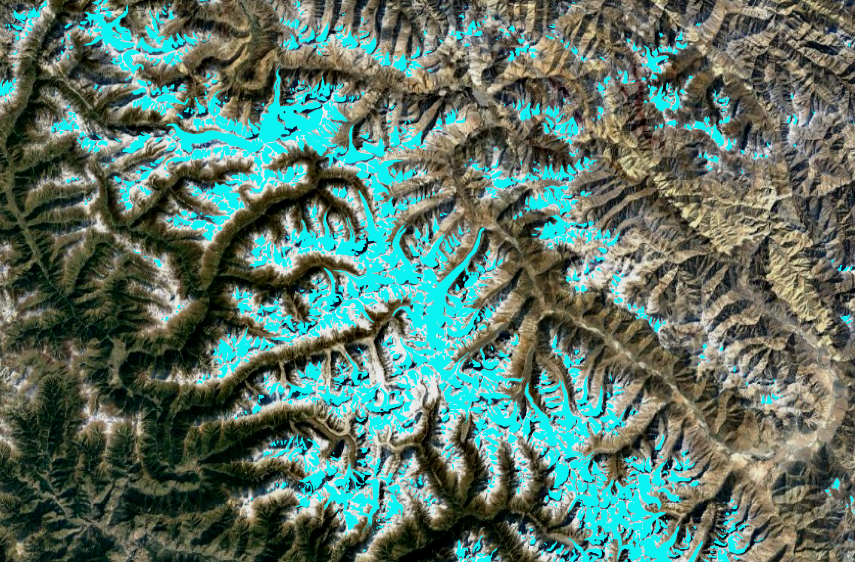
Glaciated area of the Hindu Kush Himalayas in the disputed Jammu and Kashmir area of India and Pakistan, with clean-ice glaciers (training labels) shown in blue over Google Satellite data (2021).
Deep Learning on Ice: Architecture Experiments in the Himalayan Cryosphere
This project uses experiments and visualizations to explore the "U-Net" architecture in deep learning, focusing on remote sensing applications. It takes as a starting point the glacier segmentation work published by
Baraka et al. (2020), in which a U-Net was able to capture basic semantic information in terms of glacier-pixel classification but was later shown to have failed to capture global spatial relationships such as boundaries and connections between glaciers (
Zheng et al. 2022). Seeking to extend this precedent, especially by capturing more information in the U-Net's encoding, this project implements the "attention gates" originally proposed by
Oktay et al. (2018) to improve U-Net performance on medical image segmentation tasks. The following blog will give an overview of image-based methods for glacier monitoring (including deep-learning approaches) and a summary of Baraka and Zheng et al.'s findings, followed by further experimentation and visualizations that explore whether their glacier segmentation network's performance can be improved through the integration of attention.
(1) Introduction: Images and Glaciology in the Hindu Kush Region
The Hindu Kush Himalayan region is an area of about 4.2 million square kilometers extending across all or part of Afghanistan, Bangladesh, Bhutan, China, India, Myanmar, Nepal, and Pakistan. The mountains in this region contain concentrations of snow and glaciers unmatched in any areas on earth outside the poles, and its meltwater feeds the ten largest river systems in Asia: the Amy Darya, Indus, Ganges, Brahmaputra, Irrawaddy, Salween, Mekong, Yangtze, Yellow, and Tarim (
Bajracharya et al. 2010). This water supply is indispensable in arid ecosystems downstream, especially where agriculture depends on irrigation, and its hydrological influence is so strong as to drive atmospheric circulation, energy balance and climatic regulation across the Indian Sub-continent (
Kaushik et al. 2019). Like many mountain ranges, the Hindu Kush region is very sensitive to climate change. The glaciers it holds have experienced overall shrinkage and thinning over recent decades, which threatens various aspects of the ecology and economies of the areas below. This project applies Deep Learning methods to the study of these glaciers, starting with an overview of relevant science and history.
Tracing the variable footprints of glaciers in the Himalayas has been the project of hundreds of years. The earliest known map of the mountain range was sketched by Spanish missionary Antonio Monserrate in 1590, and the Survey of India is known to have started surveying Himalayan glaciers shortly after its establishment in 1767 (
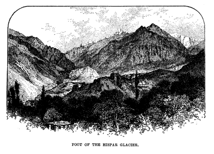
Ibid.). Subsequent nineteenth-century missions to explore and describe glacier extents, such as W.M. Conway's 1893 journey to the Hispar Glacier in present-day Pakistan, used verbal descriptions and hand-drawn images to report glacier conditions:
Conway's drawing of the Hispar Glacier, which he describes as partially clean ice and partially covered in "moraine," or glacial soil and rock deposits (
Conway 1893).
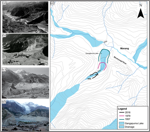
In the latter half of the twentieth century, photogrammetry and aerial photography came into widespread use for glacier sensing. Like Conway, researchers continued to use visual data to document and measure glacial extents as they appeared to onsite observers. These photographs continue to be used for long-term analysis of glacial change, such as a 2020 study that reconstructed fluctuations in the Gangapurna and Annapurna glaciers over the past 200 years using tree ring-based moraine dating and repeating photographs (
Sigdel et al. 2020). The historical photographs analyzed in this paper date back to as early as 1957 and offer a clear visual reference point in which even the layperson's eye can track changes in the location of the glacier's terminus.
Figure from Sigdel et al. with photographs showing the retreating extent of the Gangapurna glacier in 1957 (a), 1979 (c), and 2016 (b, d) and a map indicating the movement of the glacier's terminus over time (
Sigdel et al. 2020).
Concurrently with visual methods, for the bulk fo modern glaciological history, glacier mass balance has been measured using methods that involved drilling a network of stakes and pits into a glacier's surface, and then measuring the accumulation of snow and dirt at various dates across the glacial seasons of "accumulation" (snowfall) and "ablation" (melting, calving, or other reductions in mass) (
Racoviteanu et al. 2008). However, in extremely rugged and remote areas such as the Hindu Kush Himalayas, such field-based methods are at best challenging and at worst totally intractable due to the logistical complexity and risk of transporting researchers to and across the region. It is due to these difficulties that advances in the availability and resolution of remote sensing data have made a major impact on the feasibility of detailed glacier inventory in this region. In recent years, remote sensing data has facilitated the study of glacier parameters including glacier area, surface elevation, equilibrium line altitude (ELA: the area or zone on a glacier at which accumulation and ablation are equally balanced across the year), and terminus position (
Racoviteanu et al. 2008) without the deployment of in-person expeditions. It should be noted that the emergence of remonte-sensing methods for glaciology has precipitated important social consequences in the field. As
Carey et al. (2016) observe, satellite-based research approaches make possible a new form of "feminist glaciology," in which the study of glacial systems can diverge from its historical dominance by hyper-masculine polar explorers and the association of good research with highly strenuous and dangerous mountaineering missions like Conway's.
The spaceborne sensors in operation today detect solar radiation reflected by the planet's surface in the visible and near infrared bands of the electromagnetic spectrum, as well as the radiation emitted by the surface in the thermal infrared spectrum (
Ibid.). The "multi-spectral" nature of the resulting data offers new advantages beyond the information produced by historical glacier photography techniques. Multiplying the utility of this data is the density of repeated images which some satellites now capture only weeks apart, rather than decades as in
Sigdel et al. (2020).
With this new and growing volume of remote sensing data describing glaciers in the Hindu Kush region, it has become possible to apply automation workflows to the delineation of glacier extents. The feasibility of methods to do so relies on the spectral uniqueness of glacier material in several bands of the electromagnetic spectrum: snow and ice are highly reflective in visible wavelengths, less reflective in the near-infrared spectrum, and highly emissive in the thermal infrared. Unfortunately, the spectral signature of glaciers is complicated by the spectral similarity of supra-glacial debris with moraines and bedrock (
Baraka et al. 2020) This similarity, along with cloud cover, variable snow conditions, and other environmental effects can introduce errors to semi-automated mapping methodologies that are labor-intensive and time-consuming to correct. Deep learning techniques offer significant advantages for improving speed and accuracy in these processes.
The following project will explore one example of deep learning applied to glaciology, taking as its starting point the glacier segmentation model originally proposed by
Baraka et al. (2020), and later revisited by
Zheng et al. (2022). The following sections will summarize their work, explain some reduced-scale experiments relating to model-architecture modifications performed on their network, and discuss findings and potential ways forward.
(2) Glacier Segmentation U-Net: Background
The original research investigated in this project is a pixel-wise glacier segmentation network published by
Baraka et al. in 2020. It uses satellite imagery from Landsat and glacier labels for the Hindu Kush region provided by the International Centre for Integrated Mountain Development
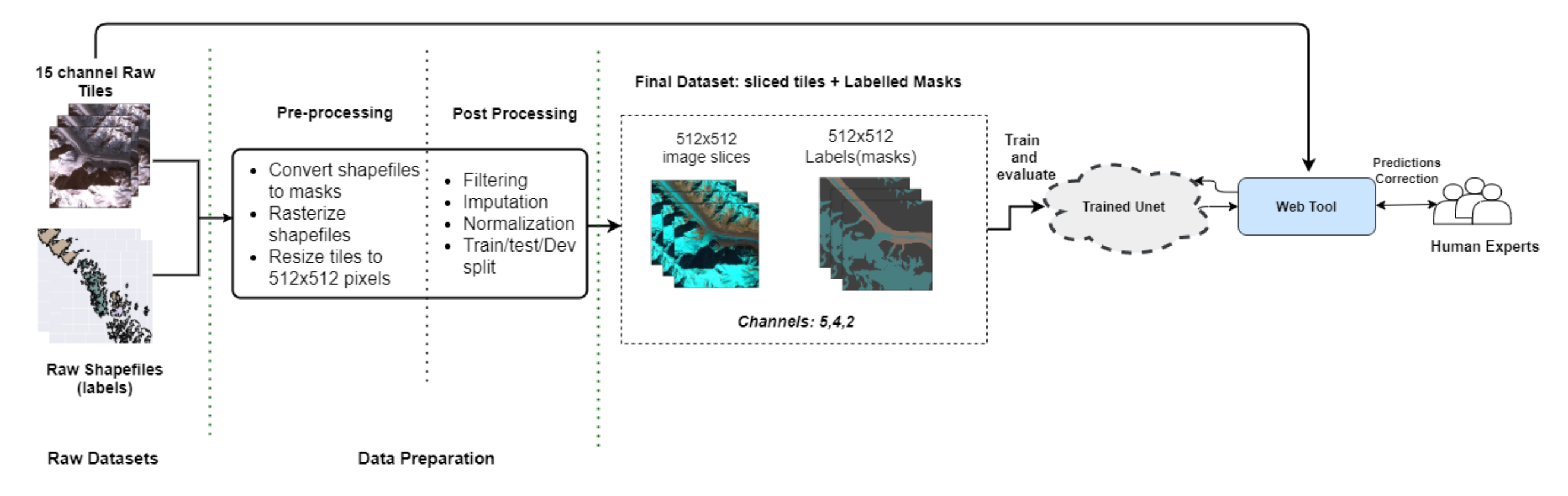
(ICIMOD) to establish baseline methods for automated glacier mapping using a U-Net deep learning architecture. This research involved the production of an intensive data pre-processing pipeline (shown below) followed by experimentation on various elements of the data and prediction workflow.
Flowchart showing research framework. Notably, the glacier segmentation results produced here are intended for use in a feeback process involving human experts (
Baraka et al. 2020).
Intervening earliest in this pipeline (preprocessing), various band selection regimes were tested to determine whether specific bands of the Landsat data were especially relevant for glacier detection. Results from this experimentation were essentially that using all of the bands considered provided better performance than limiting the data to any specific subset, though integrating elevation and slope data with the input did boost performance substantially.
Considering the middle of the workflow, further experimentation addressed the number of label classes (masks) included in the final dataset. Glaciologists are interested in both clean ice glaciers and debris-covered glaciers, which appear differently in image data: clean ice glaciers are easily confused with snow, while debris-covered glaciers can blend in with background mountain landscapes. Binary models for each type of glacier, a single binary model (glacier / non-glacier), and a multiclass model considering both types of glacier were tested. Performance was roughly similar for the single binary and multiclass models, though the multiclass approach produced better predictions in areas with higher coverage of debris-covered glaciers.
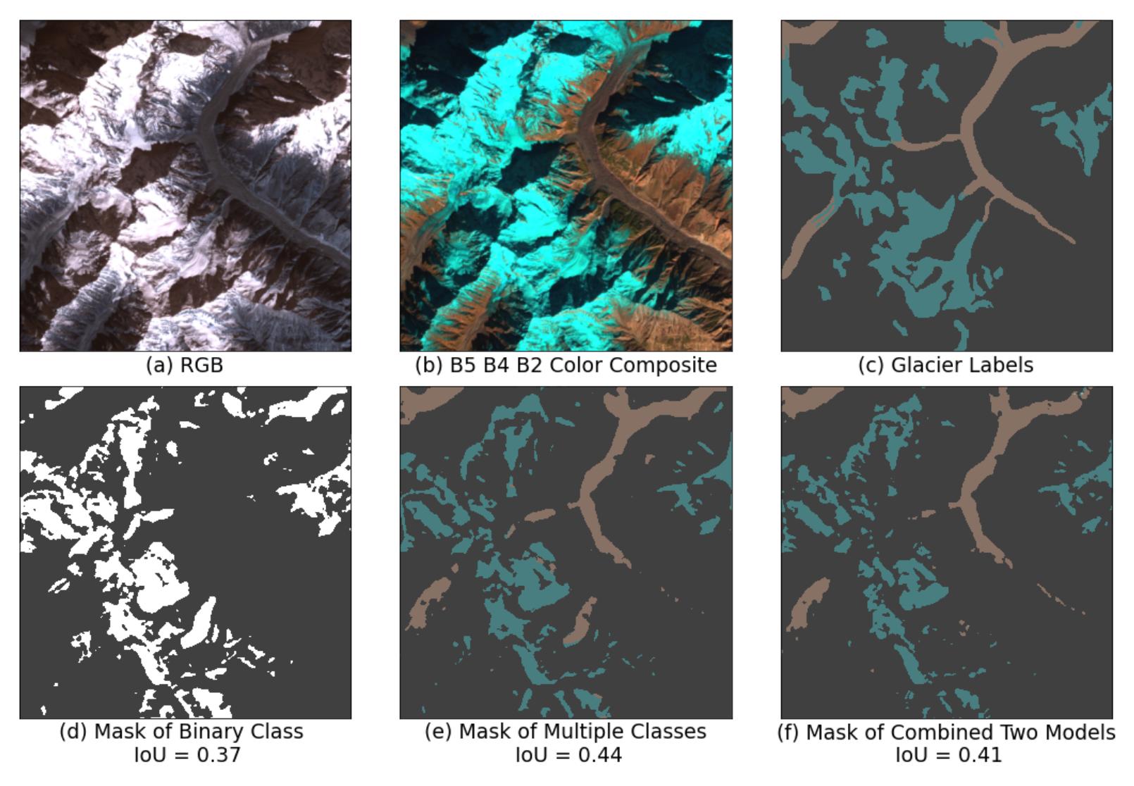
Example imagery and labels (a - c), with model predictions (d - f). Blue labels are for clean ice and brown for debris-covered glaciers. Multiclass and combined binary models give comparable predictions (e-f), but a model rained to recognize the union of clean ice or debris-covered glaciers fails to recognize major debris-covered glaciers (d). (
Baraka et al. 2020).
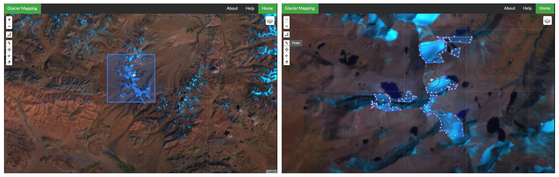
Addressing the end of the workflow, an interactive glacier mapping tool was produced to visualize the model's predictions as polygons that could be edited manually by specialists. This interactivity was intended to make the most of both model predictions and glaciologists' expert input in the service of speeding up glacier mapping workflows.
Screen Captures from the interactive web tool showing polygonized prediction for an area of interest (
Baraka et al. 2020).
(3) The U-Net Architecture
The glacier segmentation model implemented by
Baraka et al. employs a neural network architecture known as the U-Net. This architecture is commonly used in image segmentation tasks because it extends the "fully convolutional network" in such a way that fewer training images can be used to produce more precise segmentation results.
The U-Net was originally devised in 2015 by
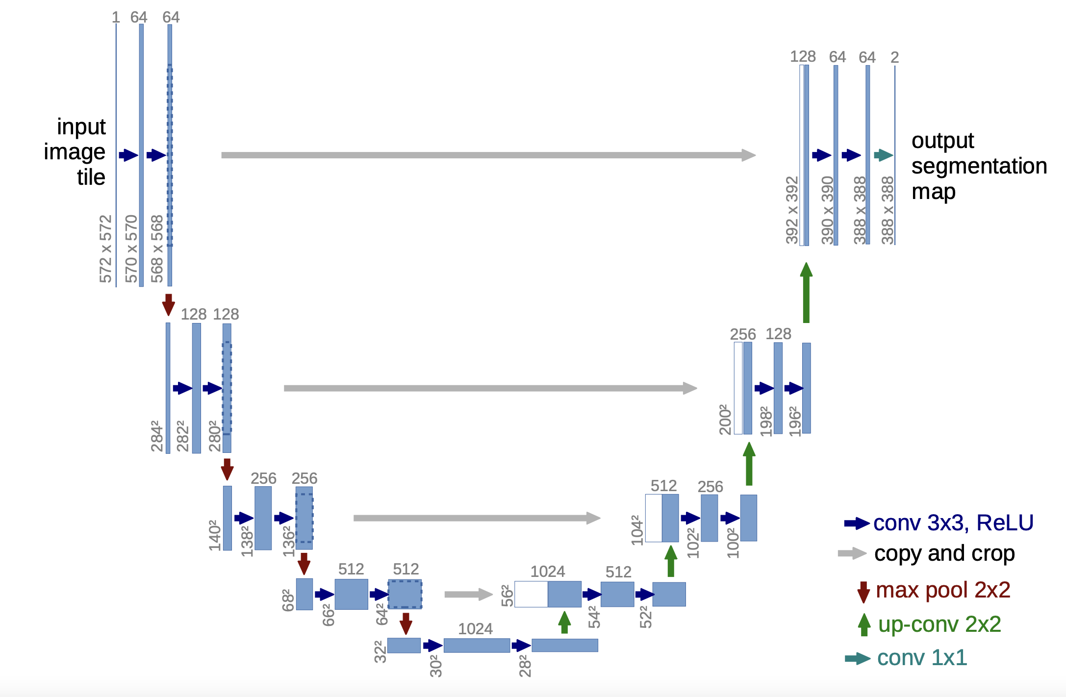
Ronneberger et al. for biomedical image segmentation tasks. The architecture is shown in a diagram below. It consists of a downsampling "contracting" or "encoder" path (left side) and an upsampling "expansive" or "decoder" path. The downsampling path follows the typical architecture of a fully convolutional network, using at each step two layers of 3x3 unpadded convolutions, each followed by a rectified linear unit (ReLU) and a 2x2 max pooling operation with stride 2. The number of feature channels is doubled at each step of the downsampling path.
Diagram of the U-Net architecture (
Ronneberger et al. 2015). Each blue box corresponds to a multi-channel feature map, with the number of channels denoted on top of the box and the x-y-size at the lower left edge of the box. White boxes represent copied feature maps. The arrows denote the different operations.
In the upsampling path, "up convolution" (transposed 2x2 convolution) layers combine up-sampling of the feature map with 2x2 convolutions, halving the number of channels in each feature map. Then, skip connections are used to concatenate this upsampled result with the corresponding feature map from the downsampling path. The combined feature map then enters two 3x3 convolutional layers, each followed by a ReLU activation, as in the downsampling path. The final layer applies a 1x1 convolution to map each feature vector to the desired number of segmentation classes.
The intended advantages of this architecture are (a) resolution and (b) localization. While previous fully convolutional networks would use pooling operations to parse the output of the contracting path, the U-Net upsamples this representation back to its original resolution. In order to localize the results of this process, the skip connections integrate high-resolution features from the contracting path into the upsampling layers, so that the information bottleneck at the middle of the U-Net does not compromise the precision of the network's output. The large number of feature channels in the upsampling pathway also help the network to propagate context information to higher resolution layers.
(4) Glacier Segmentation U-Net: Performance
Zheng et al. (2022) extending the research initiated by
Baraka et al. by further visualizing and analyizing the same glacier segmentation U-Net, with an eye to the interpretability of the network. Like the original paper, this second installment focuses on interactive visualization, this time not only so that glaciologists can correct errors in the model's predictions, but so that the performance of the model itself can be analyzed in detail.
Zheng et al. use the same model architecture and training data as
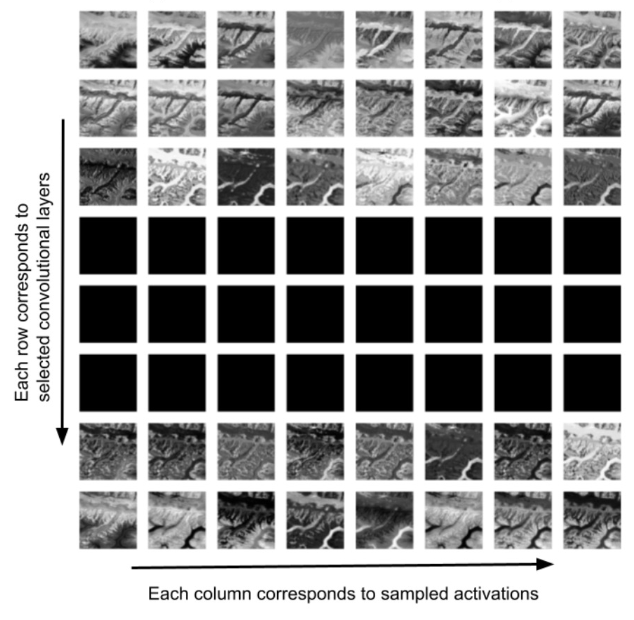
Baraka et al. but extend the interactive web visualization, allowing users to interact directly different aspects of the data which then impact prediction results in real time. However, for the purposes of exploring the U-Net architecture, the key contribution of this paper is its representation analysis of the U-Net's feature maps, layer by layer. This investigation involved passing data through the trained model and visualizing the activations it produced at individual neurons.
Activations of one satellite image for random neurons across eight convolutional layers of the U-Net model. From the top to the bottom rows, they correspond to the first, third, fifth and seventh downsampling convolutional layers, the second middle convolutional layer (bottleneck), the first and third upsampling convolutional layers and the last pooling layer.(
Zheng et al. 2022).
The above figure visualizes the results of this analysis. In reading the figure from top to bottom, it is clear that the model's learned borders between labels become clearer and more accurate during the initial down-sampling, and that these activations are recovered in the last few up-sampling layers. However, the three layers in the middle of the figure (seventh downsampling convolutional layer, middle convolutional layer, and first upsampling convolutional layer) show all black feature maps. This indicates that the information bottleneck at the middle (bottom) of the U-Net is bypassed, such that the skip connections flowing across the network provide the activations used for prediction.
Zheng et al. are not surprised by this outcome, citing recent literature that suggests that U-Net architectures struggle to learn long-range spatial relationships (for instance,
Malkin et al. observe that a landcover segmentation model misclassifies roads when they are interrupted by trees). In
Zheng et al.'s case, this failure of the model to learn any information in its deeper layers suggests that removing the middle layers could result in comparable performance with less computation. However, total reliance on skip connections for prediction output somewhat defeats the purpose of the U-Net architecture, and it leaves open an opportunity for further experimentation on this model.
(5) The Attention U-Net
Part of the issue that
Zheng et al. identified with their model was that the U-Net failed to recognize the overall shape of connected glaciers. While this kind of segmentation is fundamentally a per-pixel task, larger spatial relationships are also important: glaciers have multiple arms that are connected, and an ideal model would capture those long-distance shapes. Simultaneously, glaciers are highly variable in terms of shape and size, so this ideal model would also flexibly attend to regions of interest in input data without assuming a particular form or scale.
Similar motivations inspired the development of a new architecture by
Oktay et al. (2018), who like their predecessors
Ronneberger et al. published U-Net innovations intended for use in medical image segmentation.
Oktay et al. sought to reduce the redundant use of computational resources and parameters in preceding architectures by developing a model that could focus on relevant structures in medical imagery (in their case, the pancreas, selected for its low tissue contrast and high shape/size variability) without additional supervision. Their solution taks the form of attention gates, which serve to highlight salient features for a given task without introducing substantial computational overhead or additional parameters. Thus, attention gates improve model sensitivity and accuracy for pixel-wise label predictions by suppressing feature activatiosn in irrelevant regions.
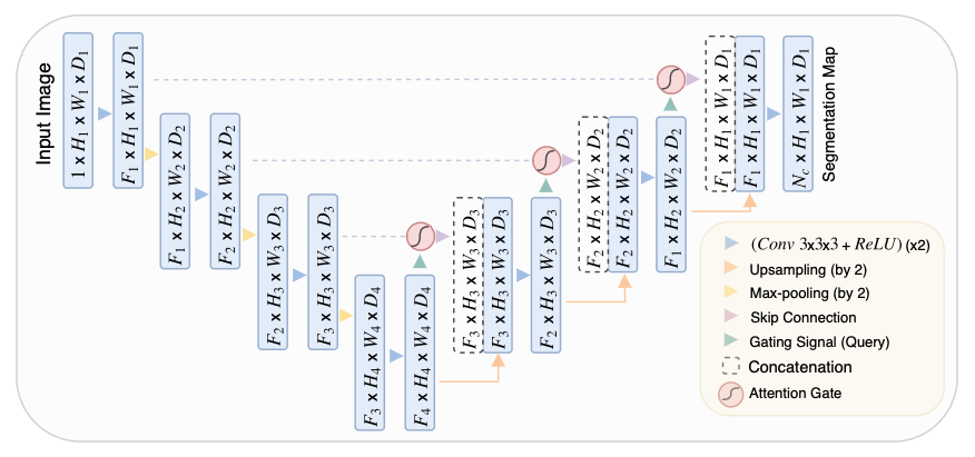
Below is a diagram of the "Attention U-Net" architecture proposed by
Oktay et al..
The downsampling path of the Attention U-Net is the same as that originally proposed by
Ronneberger et al. and later implemented by
Baraka et al. and
Zheng et al.. The difference is that at each layer of the upsampling path.
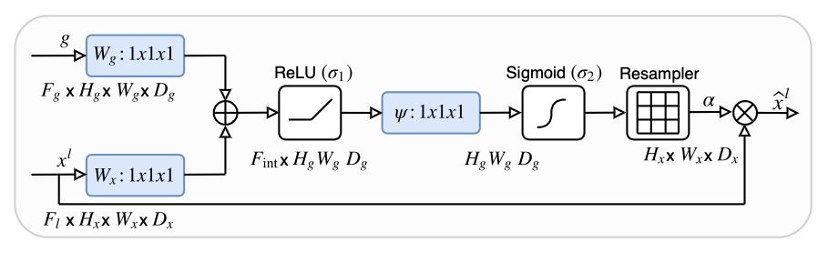
The key advantage presented by the Attention U-Net is its filtration of the features brought across the network by skip connections. Without attention, these connections introduce irrelevant low-level feature extractions from the downsampling path into the upsampling path. To do this, the attention gates assign attention coefficients (weights) to salient image regions that, when multiplied with an input feature map, preserve only the activations relevant to areas of interest for the task at hand. The gating coefficient is obtained using an "additive attention" approach.
Schematic diagram of an attention gate that selects regions of interest using the activations and contextual information from "g", which comes from one layer below the attention gate in the downsampling path.
Attention gates take in two inputs: the feature map transmitted by a skip connection ('x') and the feature map produced by the previous (that is, next lower) layer of the U-Net ('g'). Convolutions are applied to both inputs, and then they are summed element-wise such that the features that align in the two inputs are exaggerated while unaligned features are suppressed. The resulting vector is then passed through a ReLu activation layer, another 1x1 convolution, and a sigmoid activation, producing a vector of attention coefficients scaled to the range [0,1], where higher weights correspond to more relevant features. Finally, those coefficients are upsampled to the original dimensions of the skip connection feature map ('x') and multiplied with it element-wise, effectively scaling it according to relevance. The skip connection is then concatenated into the next layer as usual.
(6) Experiments
Approach
The success of
Oktay et al.'s Attention U-Net for image segmentation appears well-suited to the challenges
Zheng et al. identified in the Glacier Segmentation U-Net: while the glacier model struggled to capture the overall shape of glaciers with many connected parts, the Attention U-Net was designed to focus activations around areas known to be relevant, increasing the model's "awareness" of adjacent features.
Based on this observation, the following experiments test the hypothesis that the conversion of the glacier segmentation model to an Attention U-Net will improve its predictions. While the central problem in the existing glacier model (henceforth, the "original model") is the failure of its information bottleneck to learn any feature representations, as discovered by
Zheng et al., and attention gates only intervene in the upsampling pathway (that is, after the bottleneck), it is imagined that this approach may still help address this issue as the focusing effects of attention are transmitted backwards through backpropagation.
The experimentation described below compares a re-implementation of the original model (the "test model") to an experimental version that uses the same architecture with the addition of attention gates (the "attention model"). The models are analyzed on the basis of both their relative loss values and their respective predictions on a subset of the same glacier data from the original project.
Data
The input to both glacier segmentation models is LANDSAT tiles downloaded from Google Earth Engine and converted to cloud-optimized geotiffs. The labels are binary masks classifying glacier pixels, derived from shapefiles of glacier extents provided by
ICIMOD. Various steps of preprocessing are necessary to prepare the data for training.
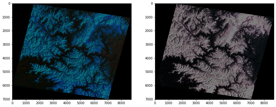
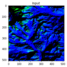
The LANDSAT tiles are geographically very large (roughly 180 km per side), and originally they contain 15 channels including the visual, near infrared, shortwave infrared, and thermal infrared spectra, as well as indices for vegetation, snow, water, elevation, and slope. Below one tile is visualized at two separate sets of channels, and its masks are shown.
At left, the tile is shown with 5-4-2 (shortwave infrared 1 - near infrared - green); these are the channels used for training. At right it is shown in RGB (with no processing yet).
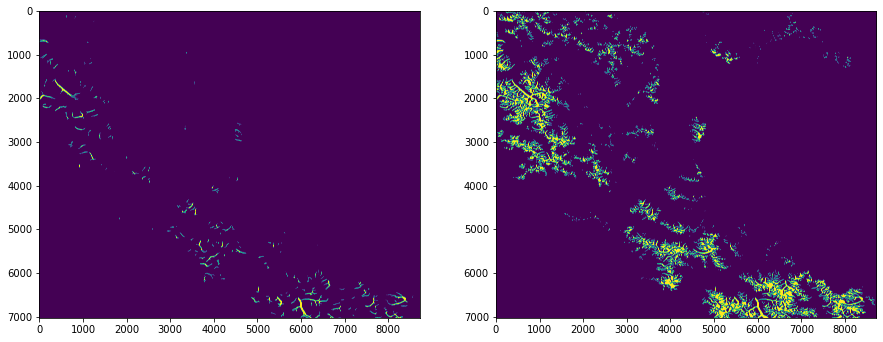
Glacier masks from ICIMOD: "debris-covered" glacier mask (left), "clean-ice" glacier mask (right).
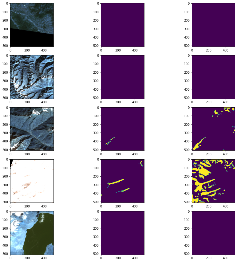
The first step of preprocessing the training data is to convert the glacier shapefiles into binary masks. Then, the LANDSAT tiles are sliced into 512x512 patches, and the corresponding binary masks are used to filter the slices so that glacier and non-glacier labels are balanced. The slices are also normalized and saved as numpy arrays at this step. Below are shown a set of slices before preprocessing.
From left to right: LANDSAT slice, "debris-covered" glacier mask, "clean-ice" glacier mask. The model is trained on a binary combination of the two masks that only differentiates glacier and non-glacier pixels.
Of the above slices, only the fourth from top would be selected for training, based on its proportion of glacier labels. It should also be noted that the LANDSAT bands (channels) used for training are the "5-4-2" channels, which correspond to shortwave infrared 1, near infrared, and green. Below is an example of a training slice after preprocessing; its colors are distorted due both to normalization and to the channels used.
Training data input slice: 3x512x512.
For this project, constraints on time and RAM made it necessary to train on only a subset of the data
Baraka et al. used. The original research used 648 training patches and 93 validation patches; this project uses 225 training patches and 33 validation patches. Luckily, the U-Net architecture is known for its applicability to tasks for which minimal training data is available!
Training
While
Baraka et al. trained the original model for 370 epochs, this project trains both the test model and the attention model for 150 epochs with a batch size of 16. Both models are trained with a binary cross-entropy loss, using the "Adam" optimizer and a learning rate of 0.0001. They also apply L1 regularization with the lambda coefficient 0.0005.
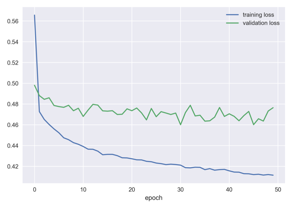
While both models trained successfully, some unexpected dynamics occurred with their respective loss functions. The first signal of confusion related to loss functions was
Zheng et al.'s loss plot, on the basis of which they describe their validation loss (green line) as converging to be "steady," which is debatable.
The validation loss above does not actually appear to have converged, even though the training loss declines smoothly.
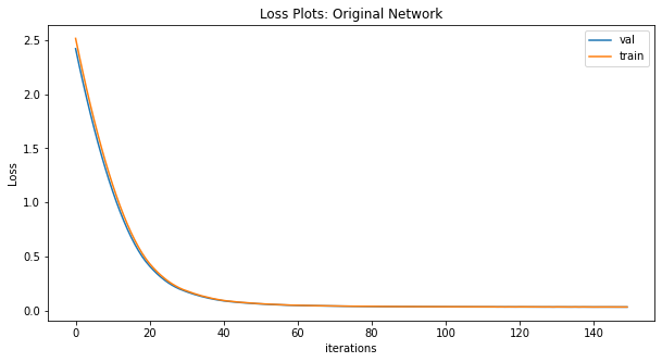
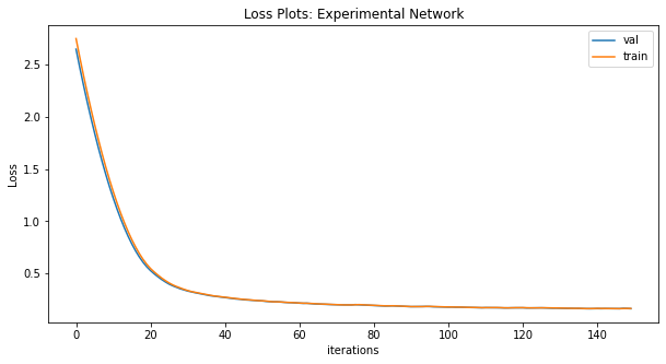
Second, using the same training loop as the original paper yielded unexpected results when training the test model and the attention model. Both loss plots show suspiciously smooth convergence, and notably the final loss values for the attention model are calculated as nearly five times higher than those of the test model. These figures are surprising given the quality of the attention model's predictions, which are explored in the next section.
By contrast with the plot above, the training and validation loss for the test model using the original training loop seems disturbingly smooth.
The training and validation losses from the experimental model look identical to
To at least calm the concerns presented by these training outputs, a manual version of the binary cross-entropy (BCE) loss was constructed and tested on the final loss outputs for each network. The results are shown below:
test final loss:
{'train': 0.03487874673945563, 'val': 0.03444354608654976}
attention final loss:
{'train': 0.16124177191938674, 'val': 0.1612364947795868}
test manual loss [val]:
0.5625313805713383
attention manual loss [val]:
0.6479246523643063
The manual BCE loss yields results that are not only different from those provided by the original training loop, but also more believable: the difference in final validation loss is much smaller (about 16% rather than 400%). While the results below suggest that both models have already converged substantially, it is also possible that the manually calculated losses would be smaller had the model been trained for 370 epochs rather than 150, as in the original research. In any case, the manually calculated losses and prediction results were accepted as a demonstration that the models had both trained correctly, in spite of the unexpected loss outputs.
(4) Results
The results of interest in this project include both the final predictions made by both experimental models and the feature maps they produced at each layer. The attention to latent outputs is important because this was the key problem
Zheng et al. identified in their network: that its predictions were acceptable, but its information bottleneck failed to learn anything during training. The discussion of experimental results for this project will start with these feature maps and then analyze both models' predictions.
Feature Maps
The key achievement of this project is its sucess at eliciting learning from the U-Net's bottleneck. Plots of the feature maps from the original model show that as
Zheng et al. demonstrated, its middle layers retain the weights assigned at initialization and fail to learn any new patterns. Meanwhile, the experimental Attention U-Net is able to produce convincing feature maps at every layer, including compelling attention maps.
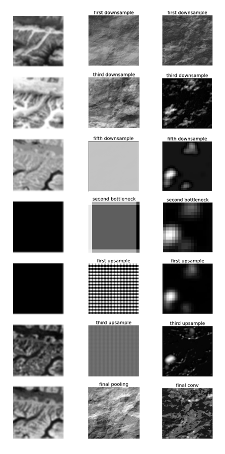
Below is shown a comparative plot of the activations from
Zheng et al. (left) alongside feature maps from the corresponding layers in the implementation of the original model (middle) and the new attention model (right).
Feature maps from corresponding layers across the original model, the test model, and the attention model. It should be oted that the input images for all three columns above are different; these feature maps are intended only to show the overall pattern in learning across the different architectures.
It is clear that the left and middle columns show an absence of learned information in the middle layers. Perhaps the addtional training epochs applied to the original model enabled legitimate activations to emerge from its fifth downsampling and third upsampling layers, while the test implmementation fails to learn anything except at the very highest level of the network. However, the key result here is that the attention model (right) succeeds in learning a specific pattern of activations at every layer in the network, indicating that information is passed through every level of the U-Net.
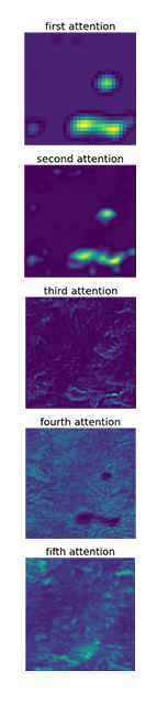
Interesting as well are the regions of interest highlighted by the attention maps in the attention model. The figures below illustrate that the attention layers identify relevant areas in their input, and that these differentiated areas remain consistent in shape across the upsampling pipeline.
Attention maps showing successfully learned soft attention.
The results offered here clearly demonstrate that the addition of attention gates to the test model makes a substantial difference in the model's ability to learn feature representations in its deeper layers.
Predictions
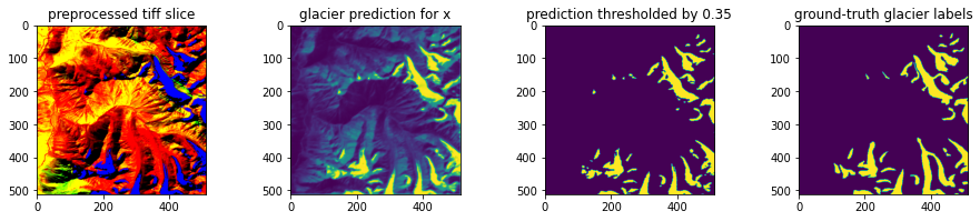
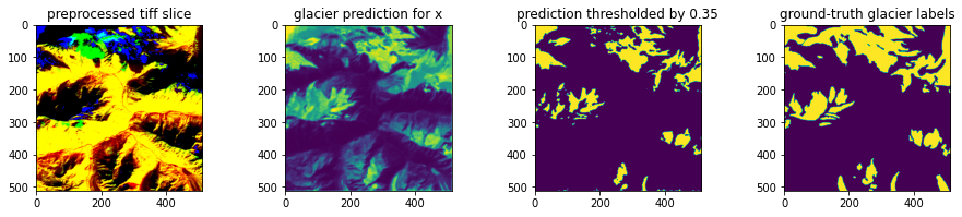
The loss values and feature maps discussed above contextualize the final predictions made by each model. Below, a set of predictions at the tiff-slice scale are visualized for each model, illustrating case studies of the various outcomes visible in output data. Click each set of figures to toggle between the test model and the attention model and assess their differences.
A: both models perform well
Test Model (U-Net)
B: both models perform well
Test Model (U-Net)
There are many examples in which both models perform well, capturing the overall shape of glacier areas as expressed in the ground-truth labels. In these cases (A and B), the attention model tends to interpret more connections between glacier segments, leading to more pixels classified as glaciers after the thresholding operation. In (B) this tendency towards more filled-out predictions brings the attention model's predictions closer to the ground truth, while in (A) it introduces some false positives that are not present in the test model's prediction. It is also noticeable that in both (A) and (B) the test model's predictions before thresholding include many more intermediate probabilities below the threshold value, while the glacier pixels identified by the attention model are more concentrated and define. This could be interpreted as an indication that the attention model is more confident than the test model in these cases.
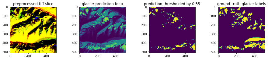
C: both models perform poorly
Test Model (U-Net)
D: both models perform poorly
Test Model (U-Net)
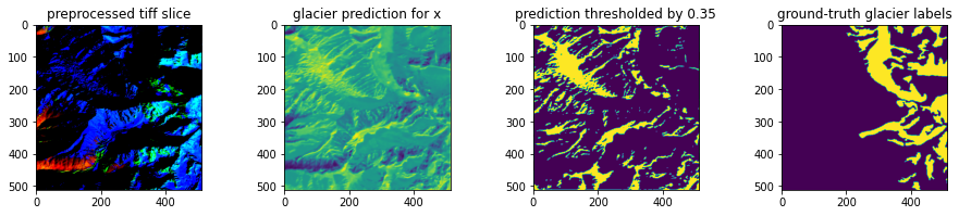
There are also many examples in which both models perform poorly, failing to recognize the distribution of glacier pixels within the frame. As in (A) and (B), in these case (C and D) the attention model tends to interpret more connections between glacier segments, leading to more pixels classified as glaciers after the thresholding operation. The above examples illustrate the worst effects of that tendency, causing glacier predictions to fill an entire slice with a pattern of false positives. The thresholded predictions in these cases look completely off-base, but the pre-threshold predictions tell a different story. Before thresholding, in both (C) and (D), the attention model's highest prediction values do align with the largest areas of glacier pixels in the ground-truth labels, while the test model fails to sense these patterns. These observations suggest that perhaps with more training (and different thresholds) the attention model could perform better on these slices.
E: attention performs better
Test Model (U-Net)
F: attention performs better
Test Model (U-Net)
Finally, there are a set of cases in which the attention model performs markedly better than the test model. In (E), the attention model's tendency to make more connected and more confident predictions allows it to more closely mimic the pattern of glaciation in the ground-truth labels, while the test model outputs a noticeable quantity of false negatives. The same effect is clear in (F), where a connected glacier system is indicated in the top 200 pixels of the ground-truth labels, and the attention model is able to represent it as such while the test model only senses separate pixel groupings. Also in (F), both models struggle to represent the glacier fragments included on the bottom edge of the ground truth labels, which may be a side effect of the test model's tendency towards false negatives and the attention model's bias towards connected glacial systems.
(6) Conclusion
This project engaged with the long history of image-based research in glaciology and contributed to the recent development of deep learning methods for glacier segmentation. Starting with the glacier segmentation U-Net analyzed by
Baraka et al. and
Zheng et al., it identified shortcomings of the existing network demonstrated by
Zheng et al.'s visualization of the U-Net's activations, in which it was evident that the middle, or lowest, layers of the model failed to learn anything. Seeking to resolve this issue in the original U-Net's information bottleneck and also improve its ability to recognize connected glacier segments, attention gates as proposed by
Oktay et al. were tested as an addition to the model's architecture.
Visualizations of the resulting attention model's inner feature maps indicate that the addition of attention gates to the test U-Net dramatically improved upon the original architecture: while the test model replicated
Zheng et al.'s observation of an absence of learning in the inner layers, the same model with attention gates successfully learned feature maps at every layer in the architecture. Furthermore, predictions made by the test and attention models indicate that while the addition of attention biases predictions toward false positives (such that its overall accuracy remains less than the test model, as shown by their respective loss functions), it does enable the model to detect connected features and capture general glacier shapes better than its predecessor.
These results are demonstrated at a much smaller scale in terms of training data and time than the original research was able to implement. However, they align with expectations based on the literature that attention gates can improve the detection of connected shapes in computer vision tasks. They also support the hypothesis that the effects of attention gates on the U-Net architecture would impact learning in the downsampling pathway and information bottleneck through backpropagation, even though they intervene later in the data's passage through the model. Further experimentation on these topics might start with longer training time on more data, as well as a modification to the training loop addressing the unexpected loss values it calculated during these experiments.
References
Code
Glacier Segmentation U-Net 2022 (data download, model architecture):
GitHub
Glacier Segmentation U-Net 2020 (data preprocessing, model architecture, training):
GitHub
Attention U-Net implementation:
GitHub
Literature
Bajracharya, S.; Maharjan, S.; Shresta, F.; Guo, W.; Liu, S.; Immerzeel, W.; & Shrestha, B. The glaciers of the Hindu Kush Himalayas: current status and observed changes from the 1980s to 2010.
DOI: 10.1080/07900627.2015.1005731 [International Journal of Water Resources Development] 6 January 2015.
Baraka, S.; Akera, B.; Aryal, B.; Sherpa, T.; Shresta, F.; Ortiz, F.; Sankaran, K.; Ferres, J.; Matin, M.; Bengio, Y. Machine Learning for Glacier Modeling in the Hindu Kush Himalaya.
arXiv:2012.05013v1 [cs.CV] 9 Dec 2020
Carey, M.; Antonello, A.; Rushing, J. Glaciers, gender, and science: A feminist glaciology framework for global environmental change research.
DOI: 10.1177/0309132515623368 [Progress in Human Geography] 2016.
Kaushik, S.; Joshi, P. K.; Singh, T. Development of glacier mapping in Indian Himalaya: a review of approaches
DOI: 10.1080/01431161.2019.1582114 [International Journal of Remote Sensing] 2019.
Malkin, N.; Ortiz, A.; Robinson, C.; Jojic, N. Mining self-similarity: Label super-resolution with epitomic representations.
arXiv:2004.11498 [cs.CV] 13 Dec 2021.
Oktay, O.; Schlemper, J.; Le Folgoc, L.; Lee, M.; Heinrich, M.; Misawa, K.; Mori, K.; McDonagh, S.; Hammerla, N.; Kainz, B.; Glocker, B;, Rueckert, D. Attention U-Net: Learning Where to Look for the Pancreas.
arXiv:1804.03999v3 [cs.CV] 20 May 2018.
Racoviteanu, A.E.; Williams, M.W.; Barry, R.G. Optical Remote Sensing of Glacier Characteristics: A Review with Focus on the Himalaya.
https://doi.org/10.3390/s8053355 [Sensors] 2008.
Ronneberger, O.; Fischer, P.; Brox, T. U-Net: Convolutional Networks for Biomedical Image Segmentation.
DOI: 10.1007/978-3-319-24574-4_28 [international Conference on Medical Image Computing and Computer-Assisted Intervention] 2015.
Racoviteanu, A.E.; Williams, M.W.; Barry, R.G. Optical Remote Sensing of Glacier Characteristics: A Review with Focus on the Himalaya.
https://doi.org/10.3390/s8053355 [Sensors] 2008.
Zheng, M.; Miao, X.; Sankaran, K. Interactive Visualization and Representation Analysis Applied to Glacier Segmentation. ISPRS Int. J. Geo-Inf. 2022, 11, 415.
https://doi.org/10.3390/ijgi11080415 22 July 2022.